Lecture 7 - Convolutional Neural Networks and Recurrent Neural Networks

Convolutional Neural Networks and Recurrent Neural Networks

Chadi Helwe, PhD

CSC 464: Deep Learning for Natural

Language Processing

Introduction

CNNs and RNNs

Deep Learning

Unlike symbolic AI or classical ML, which often use sparse, discrete representations (like one-hot encoding), Deep Learning relies on dense, continuous vectors.

Deep Learning is a class of machine learning algorithms that uses multiple layers to progressively extract higher-level features from raw input.

It defines a hierarchy of concepts: complex concepts are defined in terms of simpler ones.

CNNs and RNNs

Hierarchical Representation Learning

Deep Learning is fundamentally about representation learning.

Each successive layer builds upon the representations of the previous layer.

Example in Vision: Pixels $\rightarrow$ Edges $\rightarrow$ Textures $\rightarrow$ Object Parts $\rightarrow$ Whole Objects.

Example in Text: Characters/Sub-words $\rightarrow$ Words $\rightarrow$ Syntactic Structures $\rightarrow$ High-level Semantics.

CNNs and RNNs

Why we Didn't have Deep Learning Sooner?

For many reasons:

Hardware Limits: Deep networks require massive matrix multiplications that CPUs are too slow to handle effectively.
The Vanishing Gradient Problem: As errors are backpropagated through many layers, gradients often shrink exponentially, meaning early layers learn extremely slowly (or not at all).
The Exploding Gradient Problem: Conversely, gradients can grow exponentially, leading to numerical instability and model divergence.

CNNs and RNNs

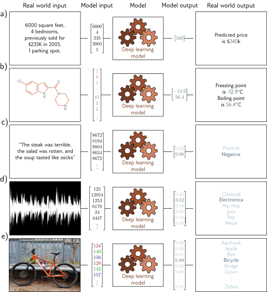
Endless Possibilities: Application of Deep Learning

CNNs and RNNs

Machine Learning vs. Deep Learning

Aspect	Machine Learning	Deep Learning
Feature Engineering	Requires manual feature extraction	Learns features automatically
Model Complexity	Simpler models (e.g., decision trees, SVM)	Complex models (deep neural networks)
Data Requirement	Works with small to medium datasets	Needs large amounts of data
Interpretability	Easier to interpret	Often a "black box"
Training Time	Usually faster	Longer due to complex architectures
Examples	Linear regression, KNN, Random Forest	CNNs, RNNs, Transformers

Convolutional Neural Networks

CNNs and RNNs

Motivation

Our goal is to predict the class of an image (e.g, cat 🐈 or dog 🐕)

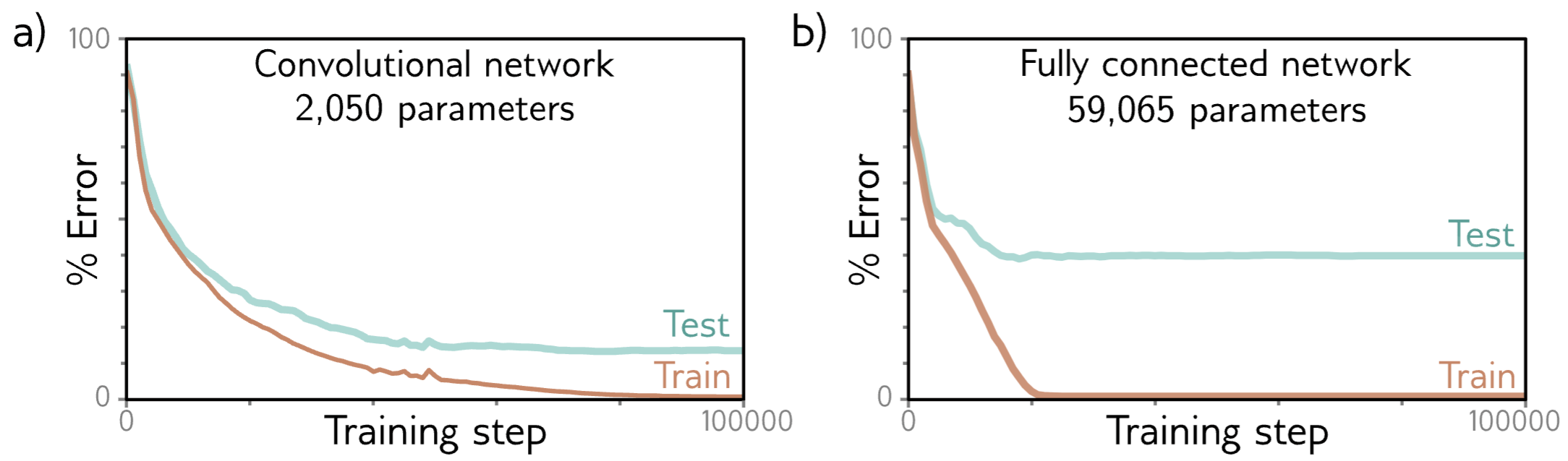
Too many parameters (slow and overfits)

Loses spatial structure (neighboring pixels matter!)

If we use a feedforward neural network:

Input = all pixels flattened into a vector.
Example: 224 x 224 x 3 = 150,528 values.
First hidden layer with 1,000 neurons → 150,528 x 1,000 ≈ 150 million weights !

CNNs and RNNs

Why Convolutional Neural Networks (CNNs)? (1/2)

Much fewer parameters + better generalization.

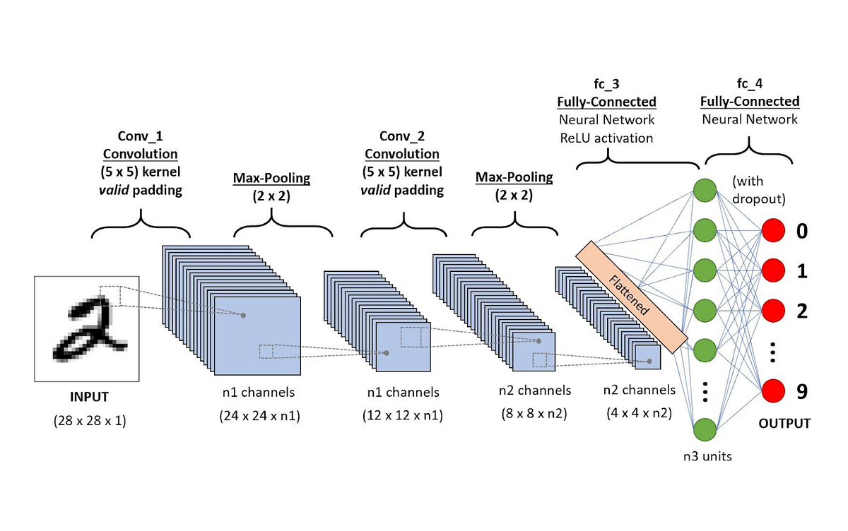
CNNs address the issues associated with using a feedforward neural network:

Local connectivity → focus on small regions at a time.
Weight sharing → same filter reused everywhere.
Spatial awareness → keeps pixel relationships.

CNNs and RNNs

Why Convolutional Neural Networks (CNNs)? (2/2)

CNNs and RNNs

Hierarchical Feature Learning

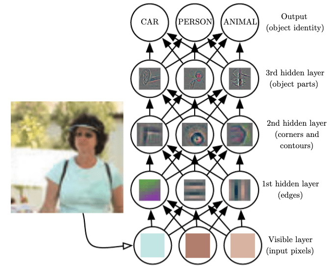
CNN layers build features step by step:

Layer 1: edges, colors.
Layer 2: corners, textures.
Layer 3+: eyes, noses, wheels, etc.
Final: full objects (cat, car, face).

CNNs and RNNs

Analogy to Human Vision

CNNs mimic this hierarchy: edges → shapes → objects.

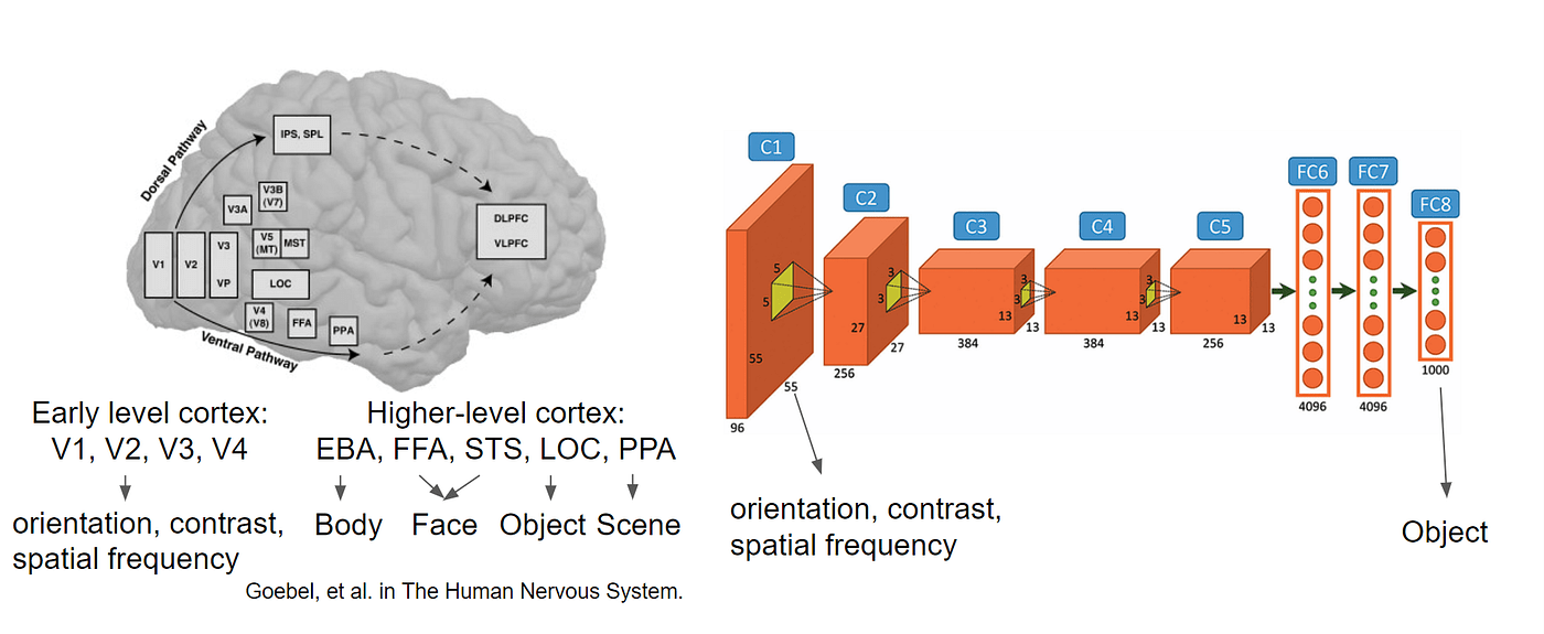
The human visual system processes local features first:

The retina detects edges, light, and motion.
The brain combines into shapes, then into full objects.

CNNs and RNNs

Convolution

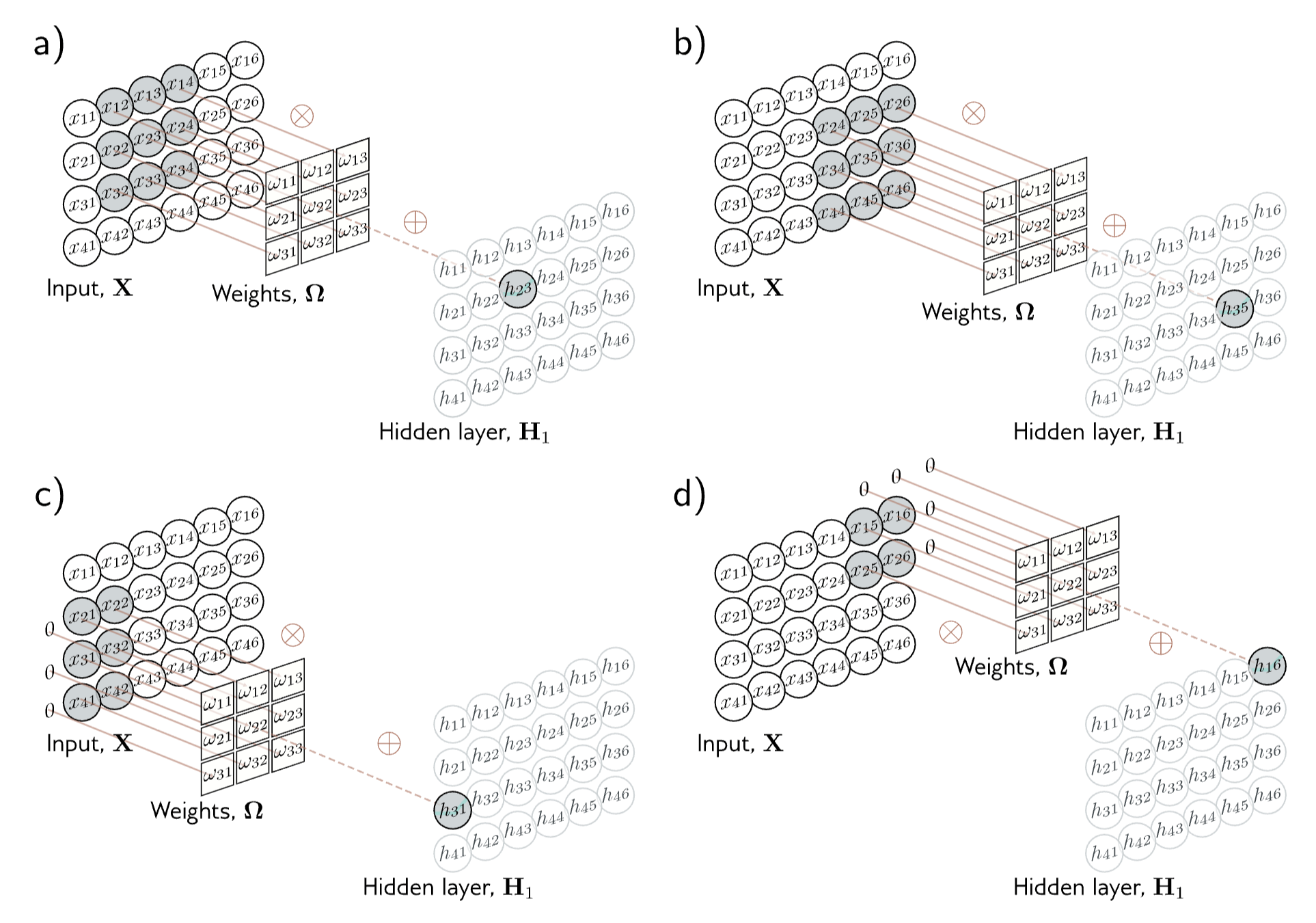
Convolution = sliding a filter (kernel) across the image.

Each filter = pattern detector (edges, textures, shapes).

Equation:

h_{ij} = \sum_{m=1}^{k} \sum_{n=1}^{k} \omega_{mn}\, x_{\,i+m-\lceil k/2 \rceil,\; j+n-\lceil k/2 \rceil}

Output = feature map → shows where pattern exists.

Feature map

Kernel size

Filter

Translation invariance: It recognizes patterns in an image regardless of where they appear in that image.

Input pixel/feature value at a shifted position. The shift term makes sure the kernel is centered.

CNNs and RNNs

Convolution Example

CNNs and RNNs

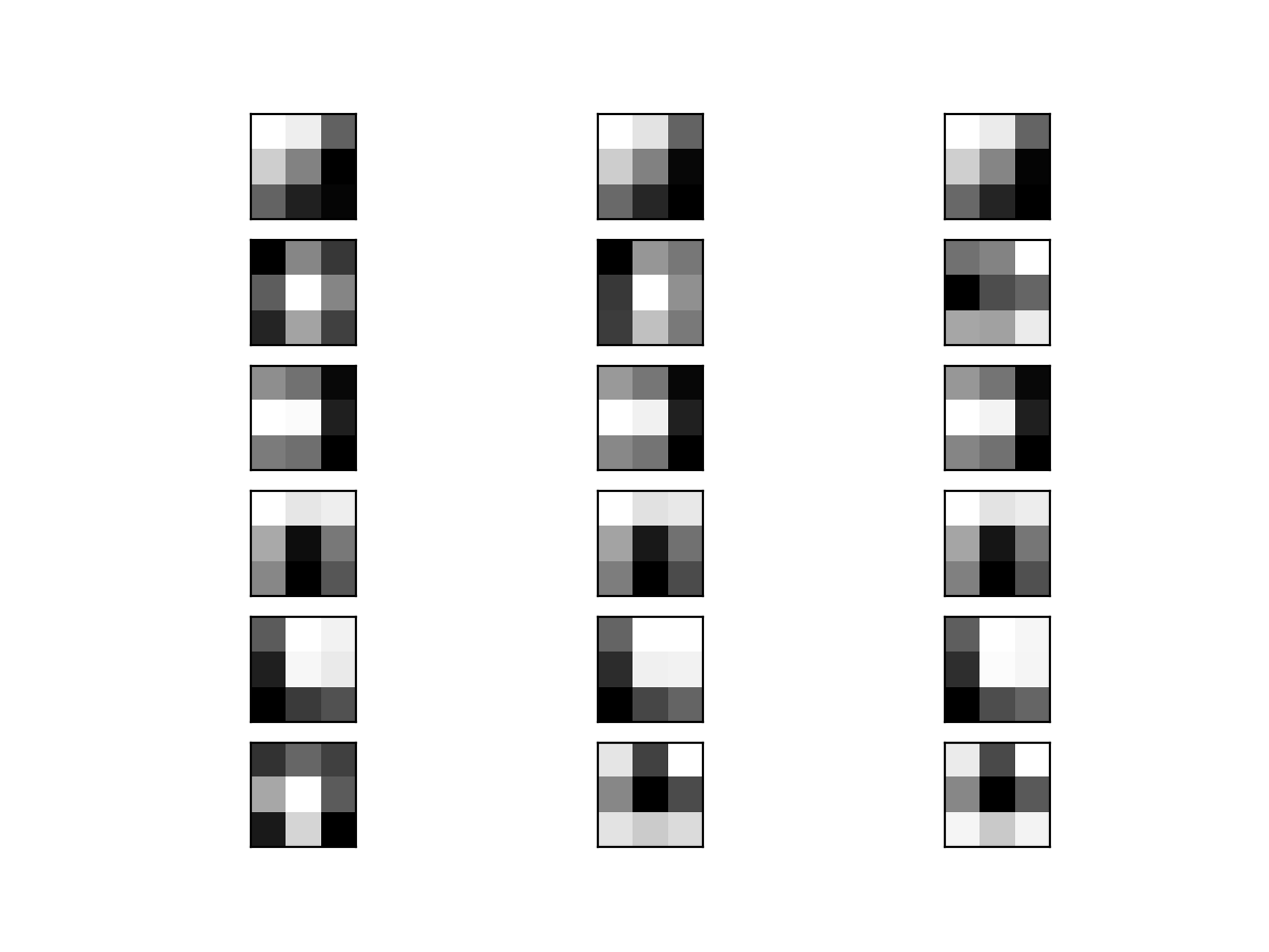
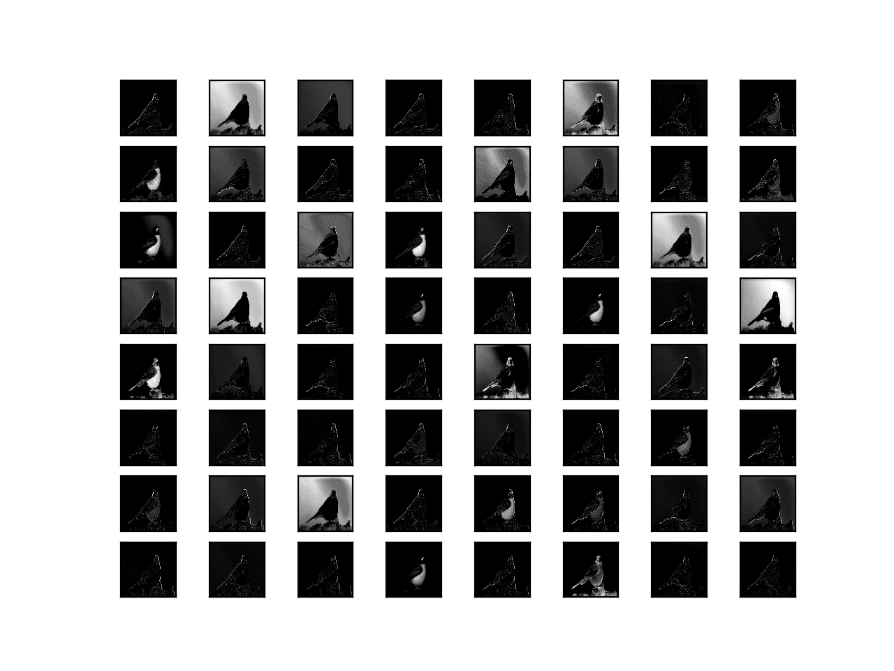
Filters in Action

Example filters:

Detect vertical edges.
Detect horizontal edges.
Detect curves.

Each produces its own feature map.

Feature Maps

Filters

CNNs and RNNs

Padding (1/4)

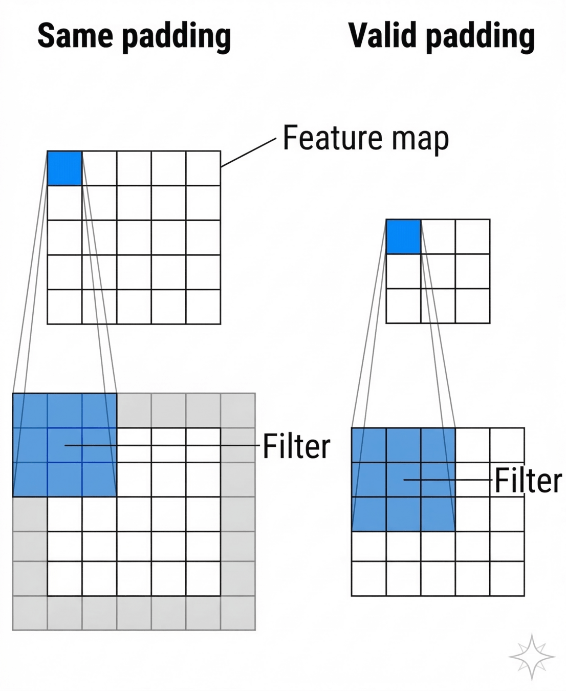
The Problem (Shrinking and Edge Loss): Standard convolutions reduce the spatial dimensions of the output feature map and under-utilize the pixels at the very edge of the input.

The Solution: Zero-Padding adds a border of zeros around the edges of the input matrix before the filter is applied, allowing the filter to center on edge pixels.

Common Padding Strategies:

Valid Padding: No padding is added. The output size shrinks (used in our earlier architecture diagram).
Same Padding: Zeros are added so the output feature map matches the spatial dimensions of the input.

CNNs and RNNs

Padding (2/4)

CNNs and RNNs

Padding (3/4)

Calculating Output Dimension ($O$):

For an input size $$N$$ , filter size $F$, padding $$P$$ , and stride $S$:

$$O = \lfloor \frac{N - F + 2P}{S} \rfloor + 1$$

To achieve "Same" padding (assuming $$S=1$$ ):

$$P = \frac{F - 1}{2}$$

Step size of the filter

CNNs and RNNs

Padding (4/4)

Example:

Given: Input $28\times28$ ( $$W=28$$ ), Kernel $5\times5$ ( $$F=5$$ ), Valid Padding ( $$P=0$$ ), Stride ( $$S=1$$ ).

Calculation:

$$O = \lfloor \frac{28 - 5 + 2(0)}{1} \rfloor + 1$$

$$O = 23 + 1 = 24$$

Result: The output feature map is exactly $24\times24$.

CNNs and RNNs

Nonlinearity (ReLU)

f(x) = \max(0, x)

Why Nonlinearity?

Without it, CNNs would just be a linear function of inputs → no complex patterns.
Nonlinear activation allows the network to learn curves, shapes, and interactions.

Use ReLU activation:

Benefits:

Introduces nonlinearity.
Makes training faster (avoids vanishing gradients).
Keeps model simple and efficient.

CNNs and RNNs

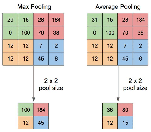
Pooling

Images/feature maps still large → need to shrink.

Max Pooling: Keeps the strongest signal in each region.

h’_{p,q} = \max \Big\{ \, h_{i,j} \;\;|\;\; (i,j) \in \mathcal{R}_{p,q} \Big\}

Benefits:

Dimensionality Reduction: Shrinks the size of the feature maps → fewer parameters → faster computation.
Translation Invariance: Distortions in the input won’t change the pooled result much.

It is a window of the input feature map that we look at to compute the output value.

CNNs and RNNs

Pooling Example

CNNs and RNNs

Fully Connected Layers

After feature extraction, CNN flattens data.

Dense layers combine features for classification.

Equation:

y = \text{softmax}(W \cdot x + b)

Output: probabilities across classes (e.g., Cat 85%, Dog 10%).

CNNs and RNNs

Putting it All Together

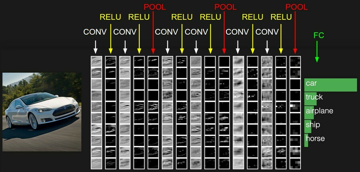
Flow:

Input image
Convolution + ReLU
Pooling
More Convs + Pooling
Fully Connected Layers
Softmax Output

CNN Architectures

CNNs and RNNs

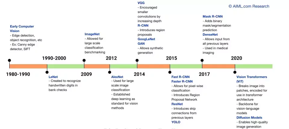
Evolution of CNN Architectures

CNNs and RNNs

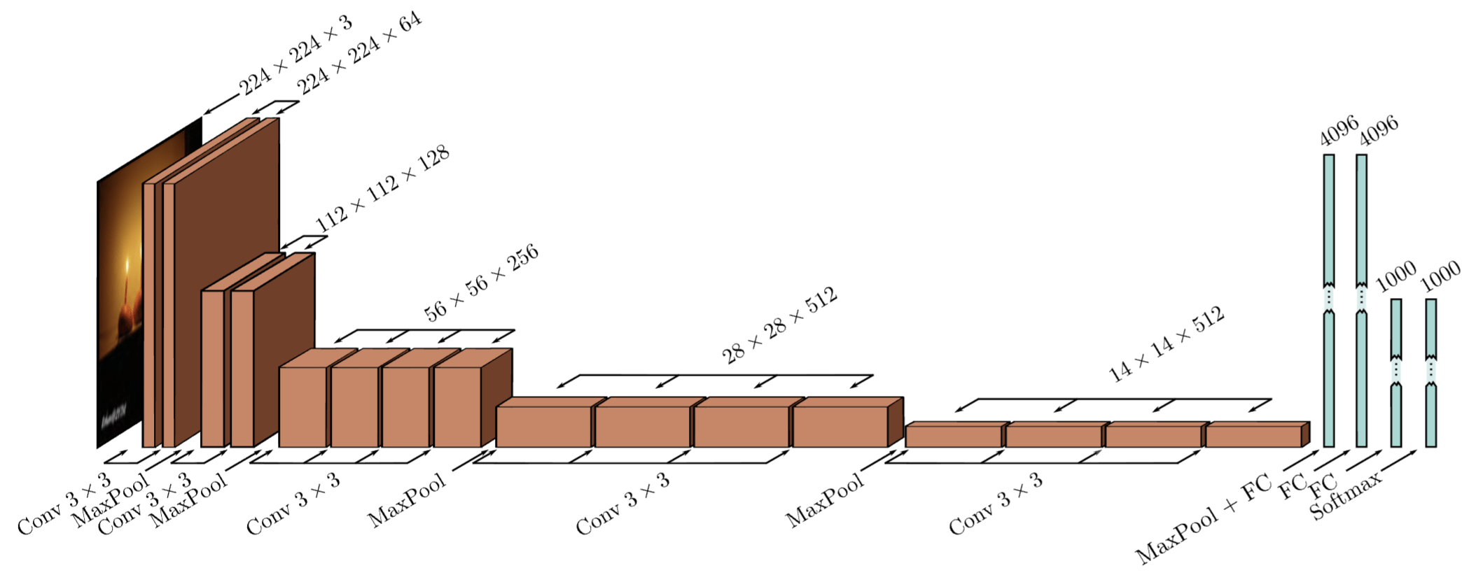
VGG: Deep but Simple

Uses 3×3 convolutional filters only, plus 2×2 pooling.

VGG16 → 13 convolutional layers + 3 FC layers

Stacking 3×3 filters ≈ larger receptive field.

CNNs and RNNs

ResNet: Key Idea

h = x + f[x, \theta]

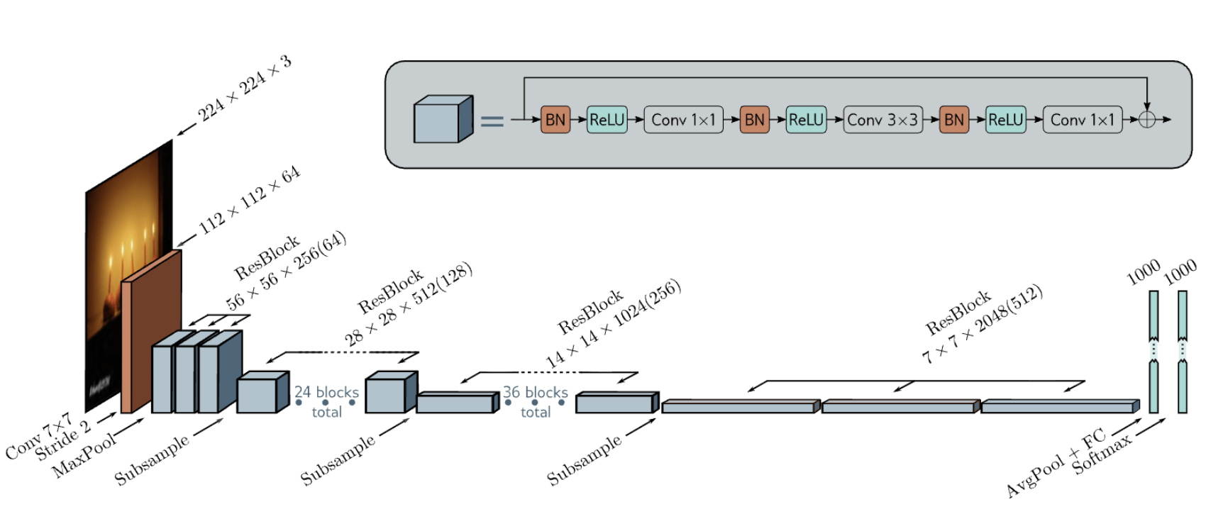
Makes gradient flow easier → train very deep networks (50, 101, 152 layers)

Problem:

Deeper networks → harder to train.
Vanishing gradients → accuracy plateaus or even drops after a certain depth.

Solution: Residual Learning

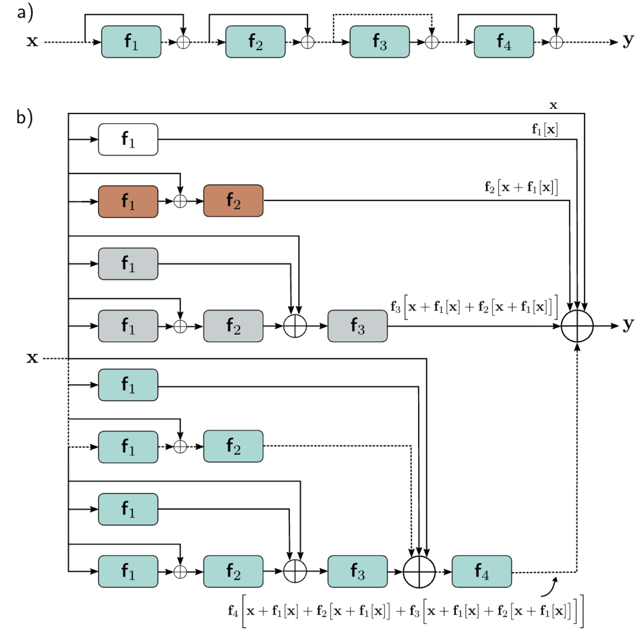
Residual or skip connections are branches in the computational paths, whereby the input to each layer is added back to the output.

CNNs and RNNs

Residual Connections

CNNs and RNNs

Why ResNet Matters?

Benefits:

Allows much deeper models to be trained successfully (50, 101, 152 layers)
Solves the vanishing gradient problem with skip connections
Improves accuracy and generalization across tasks
More efficient than VGG (fewer parameters, better performance)

CNN for NLP

Wait, CNNs for Text?

In Vision (2D): CNNs slide a 2D filter over a grid of pixels to find spatial patterns (edges, shapes, faces).

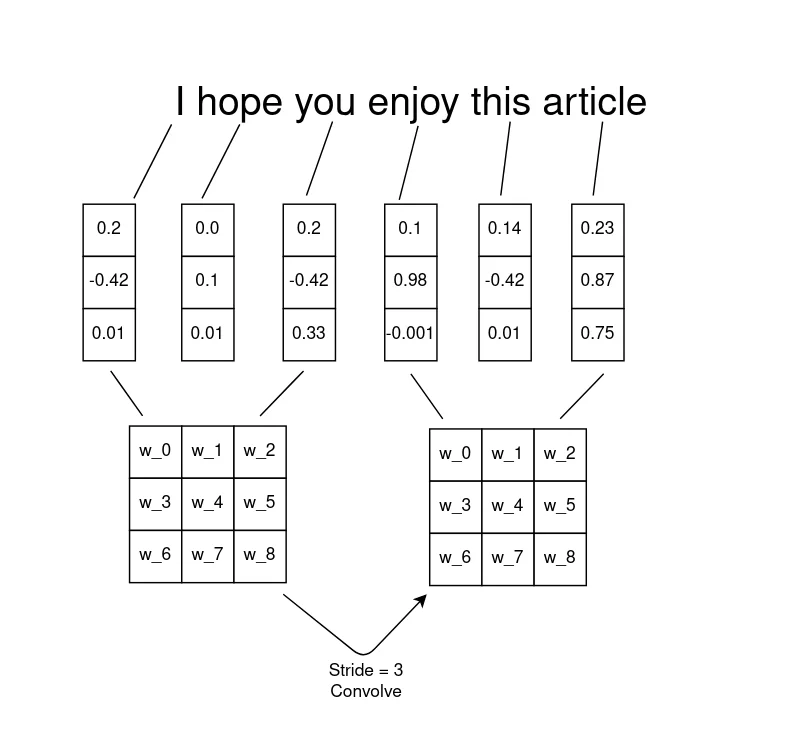
In NLP (1D): CNNs slide a 1D filter over a sequence of words to find semantic patterns (phrases, n-grams, sentiments).

CNNs and RNNs

The "Pixels" of Text

Machine learning or deep learning models cannot read raw text; they need numbers.

Embeddings: Each word is converted into a dense vector of numbers (e.g., using Word2Vec or GloVe) that captures its meaning.

The Matrix: A sentence becomes a matrix where each row is a word, and each column is a feature of that word's meaning.

CNNs and RNNs

The 1D Convolution

The Filter: A small matrix (kernel) that slides over the text matrix.

Kernel Size: Determines how many words we look at simultaneously (e.g., a size of 2 looks at bigrams, a size of 3 looks at trigrams).

Pattern Matching: The filter multiplies its weights by the word vectors to detect specific phrases (e.g., "not good", "highly recommend").

CNNs and RNNs

Max Pooling

Dimensionality Reduction: Convolutions generate a lot of feature maps. We need to shrink this data.

Global Max Pooling: For each filter, we just take the single highest value it produced across the entire sentence.

Why it works: It captures the most important feature (e.g., the strongest indicator of sentiment) regardless of where it appeared in the sentence.

CNNs and RNNs

Why Use CNNs for NLP?

Pros:

Fast and Parallelizable: CNNs can process the whole sentence at once.
Parameter Efficient: They require fewer computational resources.
Great at Local Patterns: Highly effective for tasks where a single phrase determines the outcome.

Cons:

Poor Long-Range Memory: They struggle to connect a word at the beginning of a long paragraph with a word at the end.

CNNs and RNNs

CNN Implementation for Text Classification

Loading the Data

CNNs and RNNs

from datasets import load_dataset

# Download the IMDB dataset (automatically splits into train/test)
print("Downloading IMDB data...")
dataset = load_dataset("imdb")

# Look at the structure
print(dataset)
print("\nSample Review:", dataset['train'][0]['text'][:100], "...")
print("Label:", dataset['train'][0]['label']) # 1 = Positive, 0 = Negative

Tokenization

CNNs and RNNs

from transformers import AutoTokenizer

# Load a pre-built, industry-standard tokenizer (BERT's vocabulary)
tokenizer = AutoTokenizer.from_pretrained("bert-base-uncased")

# Create a function to tokenize, pad, and truncate our text
def preprocess_function(examples):
    return tokenizer(examples["text"], 
                     padding="max_length", # Pad short reviews with 0s
                     truncation=True,      # Chop long reviews
                     max_length=500)       # Set max length to 500 words

# Apply this function to the entire dataset at blazing speed
print("Tokenizing dataset...")
tokenized_datasets = dataset.map(preprocess_function, batched=True)

Dataloaders

CNNs and RNNs

import torch
from torch.utils.data import DataLoader

# 1. Remove the raw text column (PyTorch only wants numbers)
tokenized_datasets = tokenized_datasets.remove_columns(["text"])

# 2. Tell Hugging Face to format the output as PyTorch Tensors!
tokenized_datasets.set_format("torch")

# 3. Create PyTorch DataLoaders
batch_size = 128
train_loader = DataLoader(tokenized_datasets["train"], shuffle=True, batch_size=batch_size)
test_loader = DataLoader(tokenized_datasets["test"], batch_size=batch_size)

Building the CNN

CNNs and RNNs

import torch.nn as nn
import torch.nn.functional as F

class TextCNN(nn.Module):
    def __init__(self, vocab_size, embed_dim, num_filters, kernel_size, hidden_dim):
        super(TextCNN, self).__init__()
        self.embedding = nn.Embedding(vocab_size, embed_dim)
        self.conv1d = nn.Conv1d(embed_dim, num_filters, kernel_size)
        self.fc1 = nn.Linear(num_filters, hidden_dim)
        self.dropout = nn.Dropout(0.5)
        self.fc2 = nn.Linear(hidden_dim, 1)

    def forward(self, input_ids):
        # input_ids shape: (batch_size, seq_len)
        x = self.embedding(input_ids)
        
        # Permute for CNN: (batch_size, embed_dim, seq_len)
        x = x.permute(0, 2, 1) 
        
        x = F.relu(self.conv1d(x))
        x = F.adaptive_max_pool1d(x, 1).squeeze(2)
        x = F.relu(self.fc1(x))
        x = self.dropout(x)
        return torch.sigmoid(self.fc2(x))

Training Setup

CNNs and RNNs

import torch.optim as optim

device = torch.device('cuda' if torch.cuda.is_available() else 'cpu')

# Note: We use the tokenizer's vocab size (~30,522 for BERT)
model = TextCNN(vocab_size=tokenizer.vocab_size, 
                embed_dim=128, 
                num_filters=128, 
                kernel_size=5, 
                hidden_dim=64).to(device)

criterion = nn.BCELoss()
optimizer = optim.Adam(model.parameters())

The Training Loop

CNNs and RNNs

epochs = 3 # Reduced to 3 for faster classroom execution

for epoch in range(epochs):
    model.train()
    running_loss = 0.0
    
    for batch in train_loader:
        # Hugging Face provides dicts, so we grab 'input_ids' and 'label'
        inputs = batch['input_ids'].to(device)
        labels = batch['label'].float().to(device) # BCE expects floats
        
        optimizer.zero_grad()
        
        outputs = model(inputs).squeeze(1)
        loss = criterion(outputs, labels)
        
        loss.backward()
        optimizer.step()
        
        running_loss += loss.item()
        
    print(f"Epoch {epoch+1}/{epochs} - Loss: {running_loss/len(train_loader):.4f}")

Evaluation

CNNs and RNNs

model.eval()
correct = 0
total = 0

with torch.no_grad():
    for batch in test_loader:
        inputs = batch['input_ids'].to(device)
        labels = batch['label'].float().to(device)
        
        outputs = model(inputs).squeeze(1)
        predicted = (outputs >= 0.5).float()
        
        total += labels.size(0)
        correct += (predicted == labels).sum().item()

print(f'Test Accuracy: {correct / total * 100:.2f}%')

Transfer Learning

CNNs and RNNs

Motivation

Training deep networks requires:

Large labeled datasets
Long training time

Many tasks have limited data (e.g., medical images).

Idea: Reuse pre-trained models trained on large datasets (like ImageNet).

CNNs and RNNs

What is Transfer Learning?

Definition: Using knowledge learned on one task/domain (source) to improve performance on another task/domain (target).

Example: Train on ImageNet (1M images) → reuse for medical imaging.

Works because low-level features (edges, textures) are general.

CNNs and RNNs

Approaches

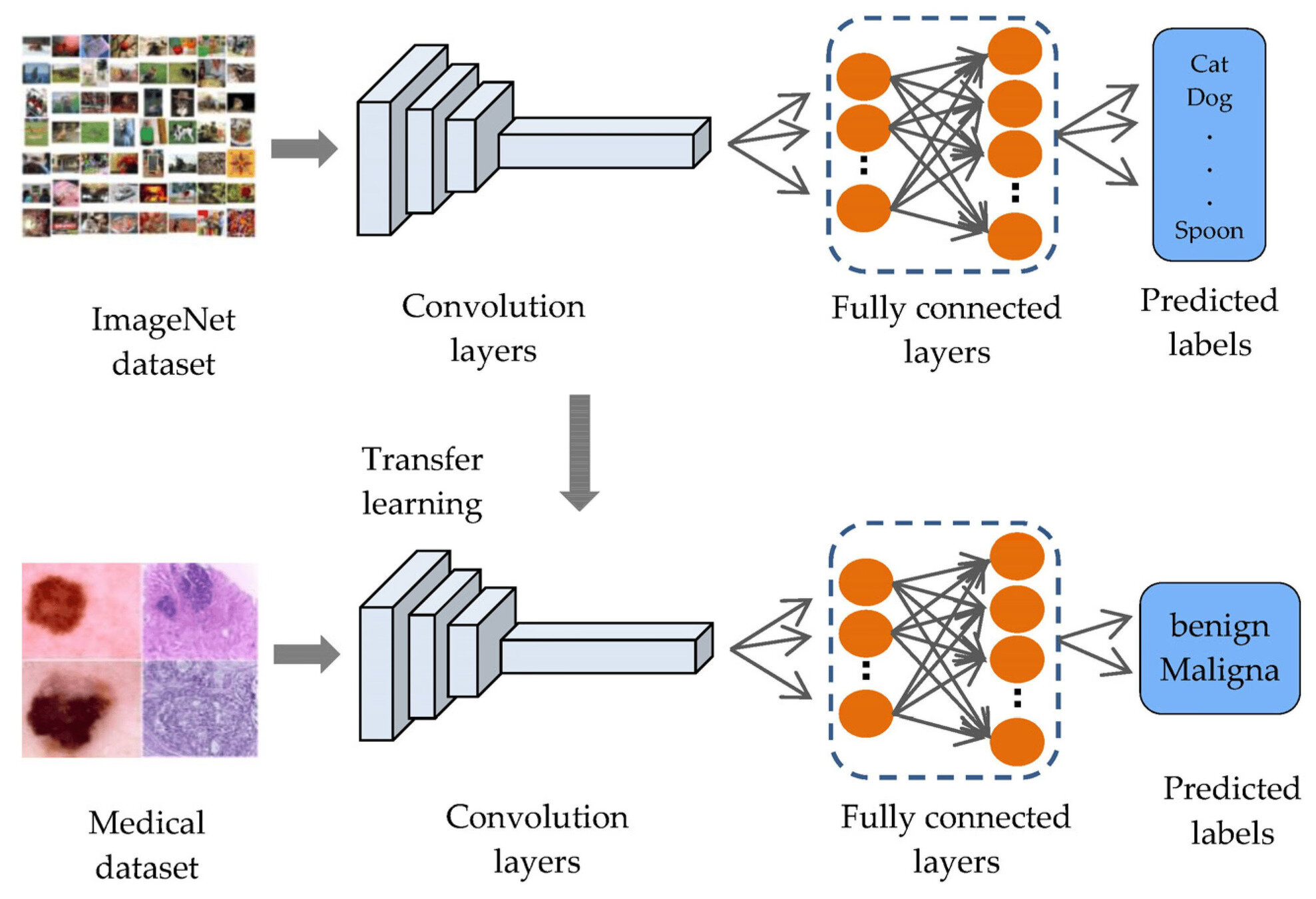
1- Feature Extraction

Freeze pretrained model
Use as feature extractor
Only train final classifier

2- Finetuning

Start with pretrained weights
Unfreeze some layers
Retrain with the new dataset

CNNs and RNNs

Benefits of Transfer Learning

1- Data Efficiency

Works well even with small target datasets.
Leverages knowledge from large pretrained models (e.g., ImageNet, GPT, BERT).

2- Faster Training

Start from pretrained weights instead of random initialization.
Reduces training time and computing cost.

3- Better Generalization

Improves accuracy compared to training from scratch.
Captures general features (edges, shapes) that transfer well.

CNNs and RNNs

Transfer Learning with ResNet-18

import torchvision.models as models
import torch.nn as nn

# Load pretrained ResNet18
model = models.resnet18(pretrained=True)

# Freeze feature extractor
for param in model.parameters():
    param.requires_grad = False

# Replace final layer for 10 classes
model.fc = nn.Linear(model.fc.in_features, 10)

Recurrent Neural Networks

CNNs and RNNs

Why Sequences Matter?

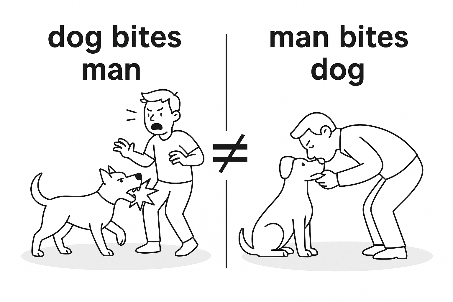
Same words, different order

→ totally different meaning

Many things in life happen in order:

Sentences in a story
Notes in a song
Daily temperatures

CNNs and RNNs

What is a Sequence?

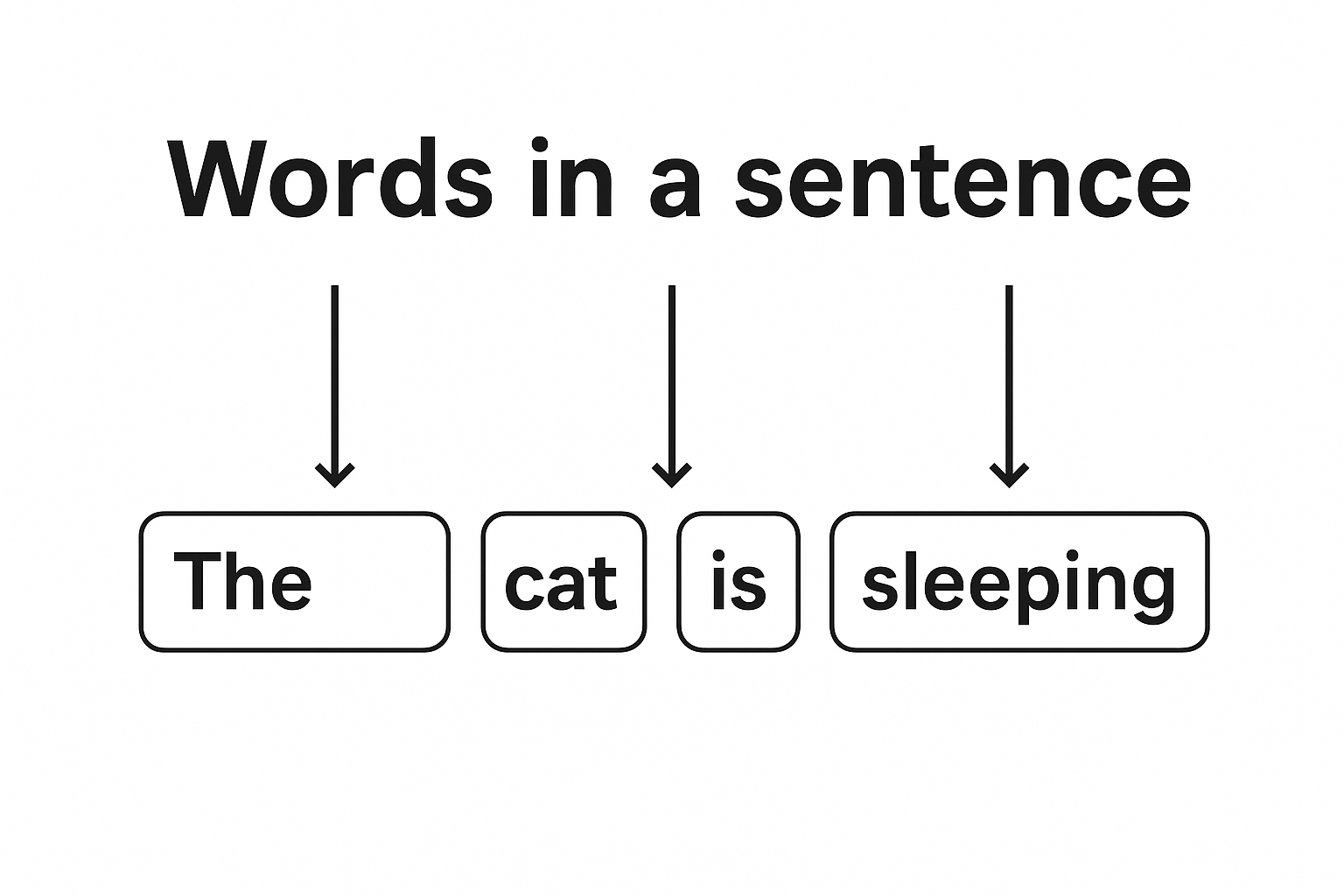
A sequence = a list of items arranged in a specific order.

Example:

Words in a sentence
Frames in a video
Steps in a recipe

CNNs and RNNs

Why FNNs Struggle with Sequences?

Fixed Input Size → Sentences can be short or long, but FNNs expect a fixed shape.

No Memory → They can’t remember past words or context.

Independent Processing → Each word is treated alone, order is ignored.

CNNs and RNNs

Introducing Sequential Models

We need models that remember what came before.

Sequential Models allow us to:

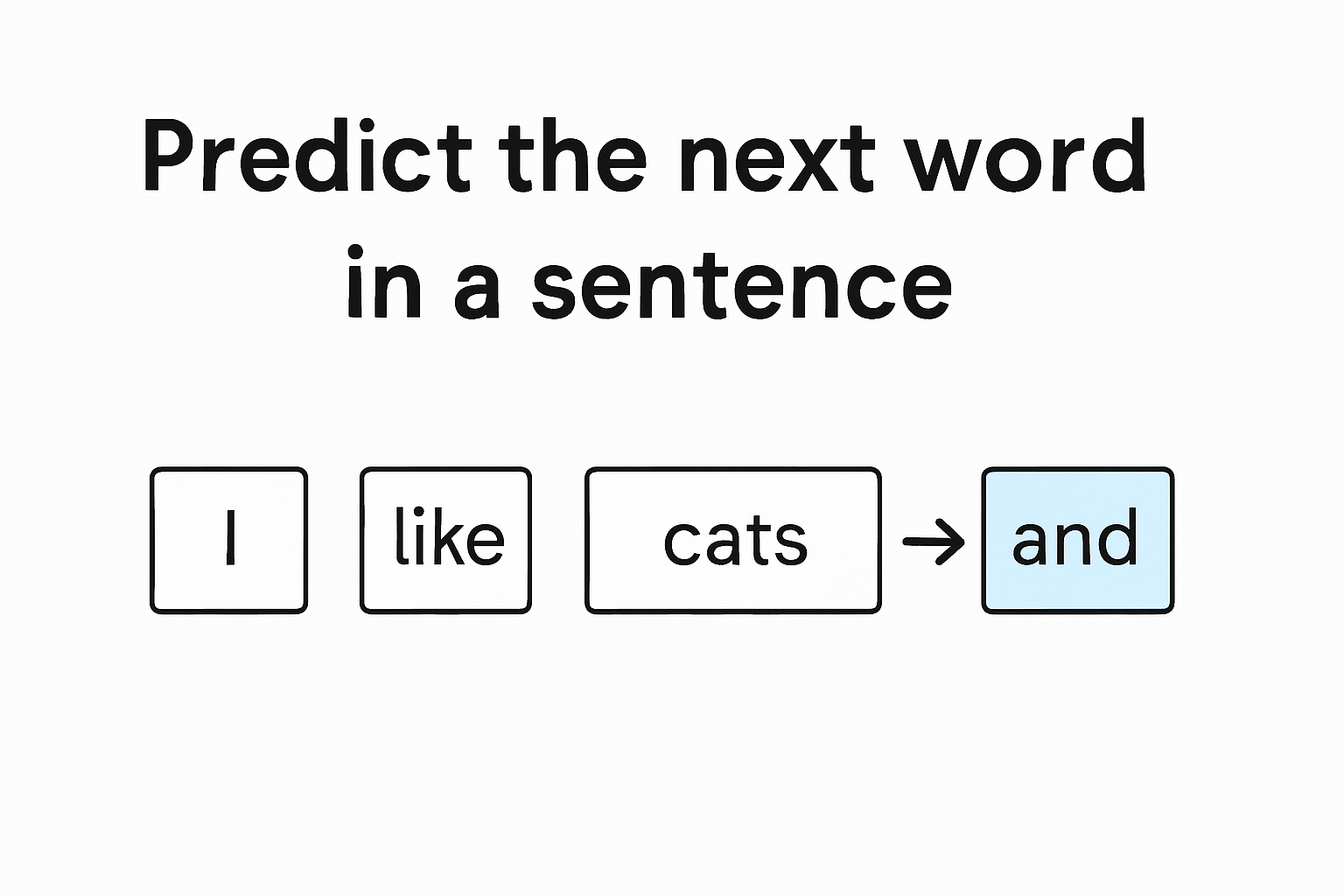
Predict the next word in a sentence
Recognize speech
Generate music

CNNs and RNNs

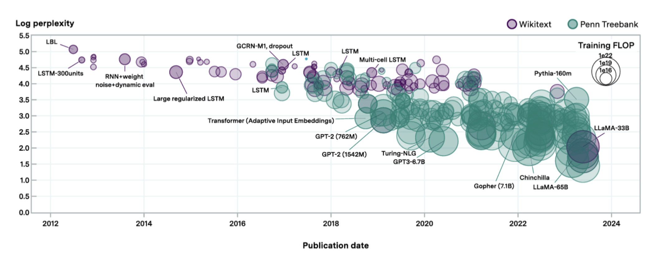
Sequential Models Timeline

CNNs and RNNs

Recurrent Neural Networks

Vanilla Recurrent Neural Networks (RNNs) are neural networks with memory. They process data step by step and keep track of what came before.

Key feature: a loop that feeds past information forward.

Equation:

h_t = f\left(W_h h_{t-1} + W_x x_t + b\right)

Hidden state (memory)

Input

CNNs and RNNs

How RNNs Work?

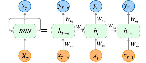
RNNs step-by-step:

Take an input (a word, a sound).
Combine it with memory from the past.
Produce an output + update the memory
Repeat this for each step in the sequence.

CNNs and RNNs

Example: Next Word Prediction

Sentence: “The cat is …”

RNN guesses: sleeping

P(\text{word}_{t+1} \mid h_t) = \text{Softmax}(W_y h_t + c)

Last hidden state

CNNs and RNNs

Strength of RNNs

Flexible with length → Can handle short or long sequences.

Context-aware → Remembers past inputs.

Order matters → Understands meaning from word order.

Versatile → Works for:

📝 Text (next-word prediction)
🎤 Speech (recognition)
🎶 Music (generation)
📈 Time-series (forecasting)

LSTMs and GRUs

CNNs and RNNs

Weaknesses of Vanilla RNNs

Equation:

$$h_t = f\left(W_h h_{t-1} + W_x x_t + b\right)$$

Weaknesses:

Forgetting long-term info (short memory).
Vanishing gradients: gradients at early layers become ≈ 0.
Exploding gradients: gradients grow too large → unstable training

✨ We need a better solution → LSTMs and GRUs

CNNs and RNNs

LSTM Neural Networks (1/3)

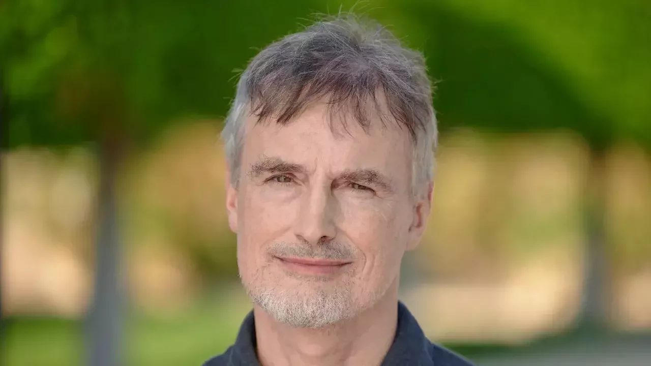
Long Short-Term Memory (LSTM) Neural Network was created by Sepp Hochreiter and Jürgen Schmidhuber in 1997.

Designed to fix RNN memory issues.

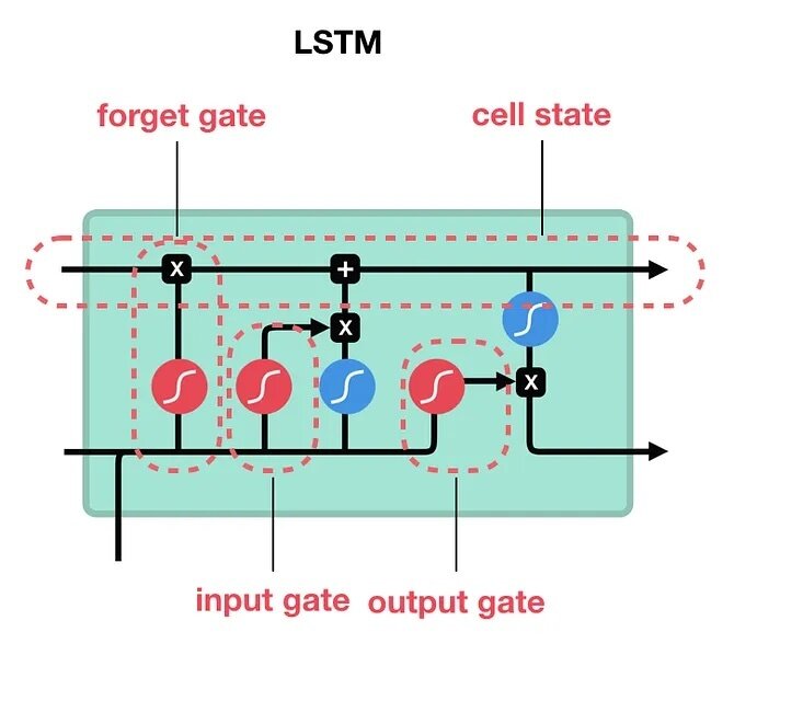
Key idea: gates control memory.

CNNs and RNNs

LSTM Neural Networks (2/3)

LSTM has two memories:

$C_t$: long-term memory (cell state)
$h_t$: short-term memory (hidden state)

Three gates control the flow

Forget gate: $f_t = \sigma(W_f [h_{t-1}, x_t] + b_f)$
Input gate: $ i_t = \sigma(W_i [h_{t-1}, x_t] + b_i) $ and $\tilde{C}t = \tanh(W_C [h{t-1}, x_t] + b_C)$
Cell state update: $C_t = f_t \cdot C_{t-1} + i_t \cdot \tilde{C}_t$
Output gate: $o_t = \sigma(W_o [h_{t-1}, x_t] + b_o)$ and $h_t = o_t \cdot \tanh(C_t)$

Gates

CNNs and RNNs

LSTM Neural Networks (3/3)

CNNs and RNNs

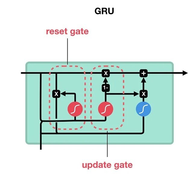
GRU Neural Networks (1/2)

Gated Recurrent Unit (GRU) Neural Network was invented in 2014.

Like LSTM, but fewer gates → faster.

Gates:

Update gate = how much to keep.
Reset gate = how much to forget.

Equation:

$$h_t = (1 - z_t) \cdot h_{t-1} + z_t \cdot \tilde{h}_t$$

New info

CNNs and RNNs

GRU Neural Networks (2/2)

LSTM Implementation for Text Classification

CNNs and RNNs

Loading the Data

from datasets import load_dataset

# Download the IMDB dataset (automatically splits into train/test)
print("Downloading IMDB data...")
dataset = load_dataset("imdb")

# Look at the structure
print(dataset)
print("\nSample Review:", dataset['train'][0]['text'][:100], "...")
print("Label:", dataset['train'][0]['label']) # 1 = Positive, 0 = Negative

CNNs and RNNs

Tokenization

from transformers import AutoTokenizer

# Load a pre-built, industry-standard tokenizer (BERT's vocabulary)
tokenizer = AutoTokenizer.from_pretrained("bert-base-uncased")

# Create a function to tokenize, pad, and truncate our text
def preprocess_function(examples):
    return tokenizer(examples["text"], 
                     padding="max_length", # Pad short reviews with 0s
                     truncation=True,      # Chop long reviews
                     max_length=500)       # Set max length to 500 words

# Apply this function to the entire dataset at blazing speed
print("Tokenizing dataset...")
tokenized_datasets = dataset.map(preprocess_function, batched=True)

CNNs and RNNs

Dataloaders

import torch
from torch.utils.data import DataLoader

# 1. Remove the raw text column (PyTorch only wants numbers)
tokenized_datasets = tokenized_datasets.remove_columns(["text"])

# 2. Tell Hugging Face to format the output as PyTorch Tensors!
tokenized_datasets.set_format("torch")

# 3. Create PyTorch DataLoaders
batch_size = 128
train_loader = DataLoader(tokenized_datasets["train"], shuffle=True, batch_size=batch_size)
test_loader = DataLoader(tokenized_datasets["test"], batch_size=batch_size)

CNNs and RNNs

Building the LSTM

import torch.nn as nn
import torch.nn.functional as F

class TextLSTM(nn.Module):
    def __init__(self, vocab_size, embed_dim, hidden_dim):
        super(TextLSTM, self).__init__()
        
        self.embedding = nn.Embedding(vocab_size, embed_dim)
        self.lstm = nn.LSTM(input_size=embed_dim, 
                            hidden_size=hidden_dim, 
                            batch_first=True)
        self.fc1 = nn.Linear(hidden_dim, 64)
        self.dropout = nn.Dropout(0.5)
        self.fc2 = nn.Linear(64, 1)

    def forward(self, input_ids):
        # Shape: (batch_size, seq_len) -> (batch_size, seq_len, embed_dim)
        x = self.embedding(input_ids) 
        
        lstm_out, (hidden_state, cell_state) = self.lstm(x)
        
        last_thought = lstm_out[:, -1, :]
        
        x = F.relu(self.fc1(last_thought))
        x = self.dropout(x)
        return torch.sigmoid(self.fc2(x))

CNNs and RNNs

Training Setup

import torch.optim as optim

device = torch.device('cuda' if torch.cuda.is_available() else 'cpu')

# Note: We use the tokenizer's vocab size (~30,522 for BERT)
model = TextLSTM(vocab_size=tokenizer.vocab_size, 
                 embed_dim=128, 
                 hidden_dim=128).to(device)

criterion = nn.BCELoss()
optimizer = optim.Adam(model.parameters(), lr=0.001)

CNNs and RNNs

The Training Loop

epochs = 3 # Reduced to 3 for faster classroom execution

for epoch in range(epochs):
    model.train()
    running_loss = 0.0
    
    for batch in train_loader:
        # Hugging Face provides dicts, so we grab 'input_ids' and 'label'
        inputs = batch['input_ids'].to(device)
        labels = batch['label'].float().to(device) # BCE expects floats
        
        optimizer.zero_grad()
        
        outputs = model(inputs).squeeze(1)
        loss = criterion(outputs, labels)
        
        loss.backward()
        optimizer.step()
        
        running_loss += loss.item()
        
    print(f"Epoch {epoch+1}/{epochs} - Loss: {running_loss/len(train_loader):.4f}")

CNNs and RNNs

Evaluation

model.eval()
correct = 0
total = 0

with torch.no_grad():
    for batch in test_loader:
        inputs = batch['input_ids'].to(device)
        labels = batch['label'].float().to(device)
        
        outputs = model(inputs).squeeze(1)
        predicted = (outputs >= 0.5).float()
        
        total += labels.size(0)
        correct += (predicted == labels).sum().item()

print(f'Test Accuracy: {correct / total * 100:.2f}%')

Convolutional Neural Networks and Recurrent Neural Networks

Introduction

Convolutional Neural Networks

CNN Architectures

CNN for NLP

CNN Implementation for Text Classification

Transfer Learning

Recurrent Neural Networks

LSTMs and GRUs

LSTM Implementation for Text Classification

Thank You