
Neural Networks
Chadi Helwe, PhD
CSC 464: Deep Learning for Natural
Language Processing
What are Neural Networks?
What are Neural Networks?
Neural Networks
Neural Networks are powerful tools that have advanced the state-of-the-art in NLP in recent years.
The foundations can be traced back to the 1940s with the work of McCulloch and Pitts (1943).
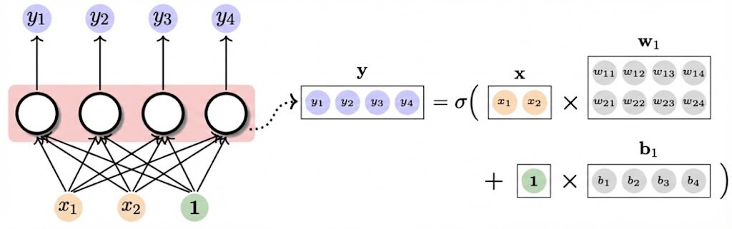
A neural network consists of small computing units that take a vector of input values and produce a single output value.
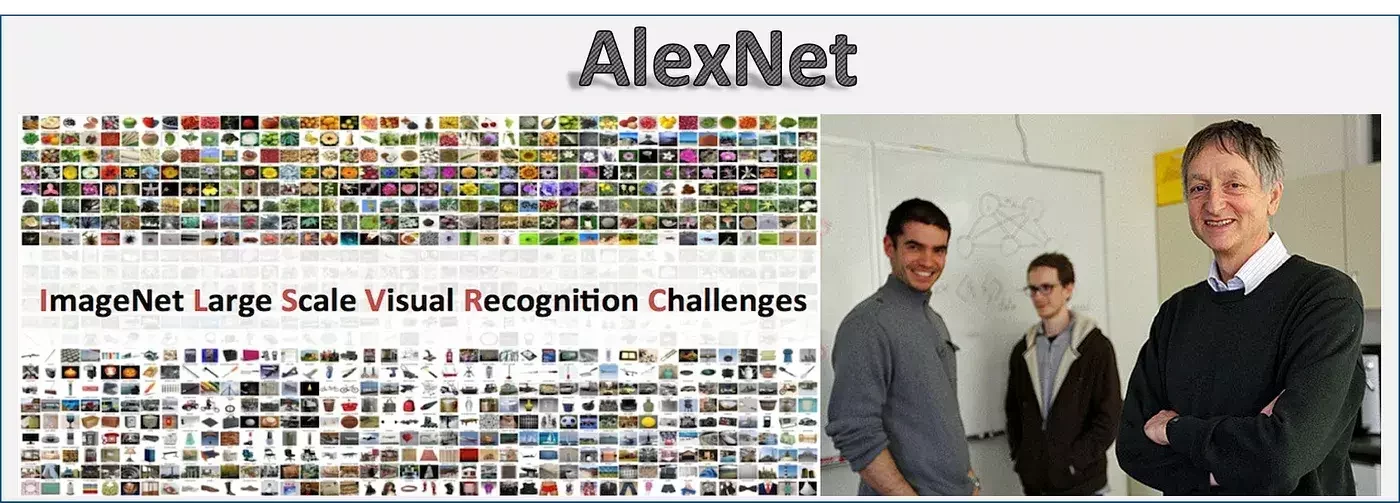
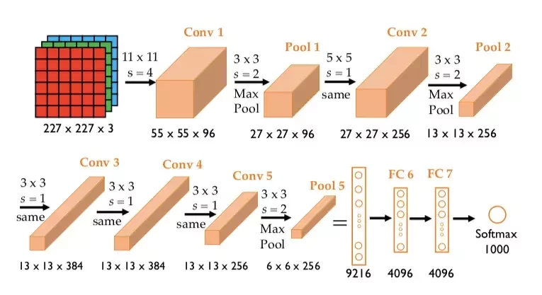
AlexNet
Neural Networks
Why Now? Three Key Ingredients
Neural Networks
-
🌊 Massive data
"Neural networks learn better when they see more examples." (Social media, sensors, internet-scale data) -
🔥 Powerful GPUs
"Faster hardware means faster learning." (Thousands of matrix operations processed in parallel) -
🧠 Better algorithms
"Breakthrough architectures and training techniques unlocked deep learning’s true potential." (ReLU activations, Adam optimizer, and Transformers)
All three together made the deep learning revolution possible.
Multi-layer Neural Networks
Neural Networks
Single-layer Perceptrons (1/2)
A single-layer perceptron (neuron) is the simplest form of a neural network. It is considered a biologically inspired program that transforms input into output, mimicking how biological neurons receive electrochemical inputs from other neurons and determine whether to pass the signal along.
Activation
Function
Weight
Input Vector
Neural Networks
Single-layer Perceptrons (2/2)
Neural Networks
Activation Functions
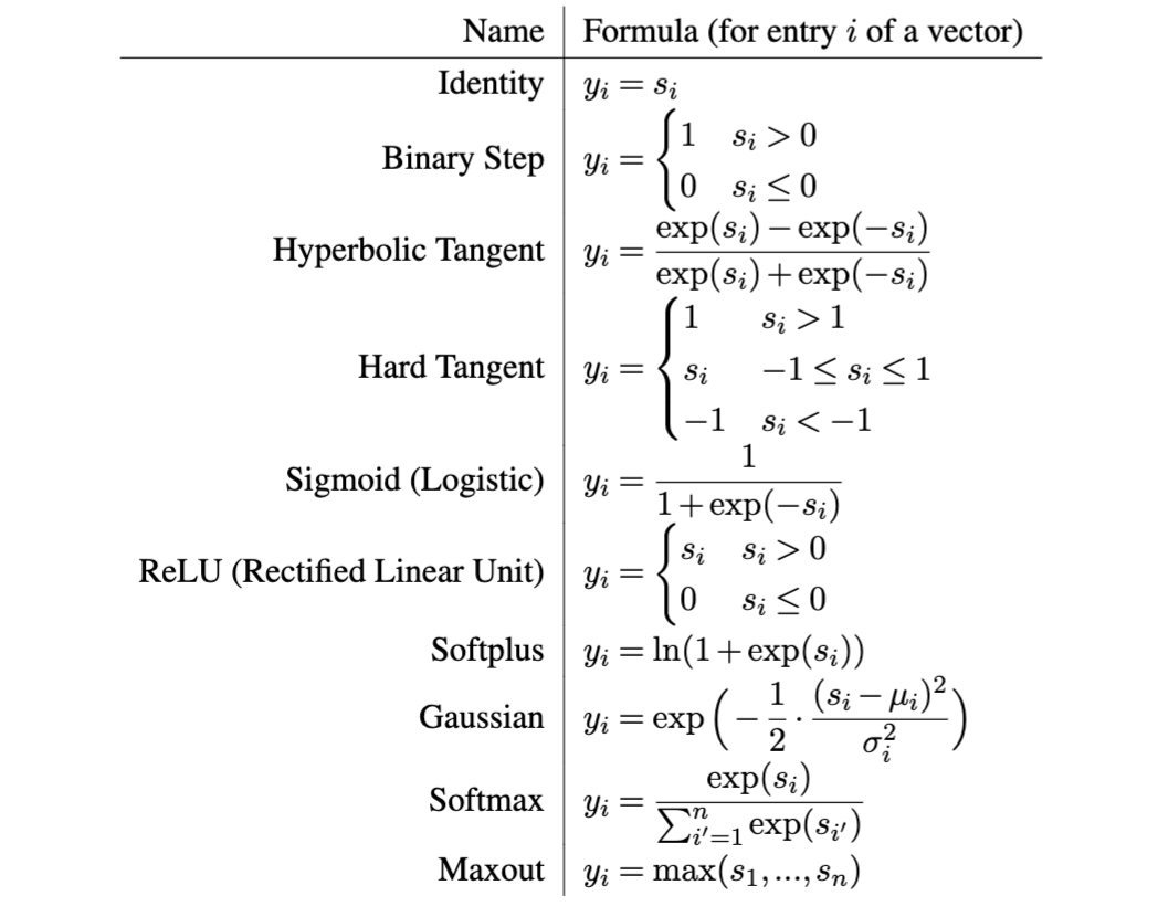
Neural Networks
Activation Functions
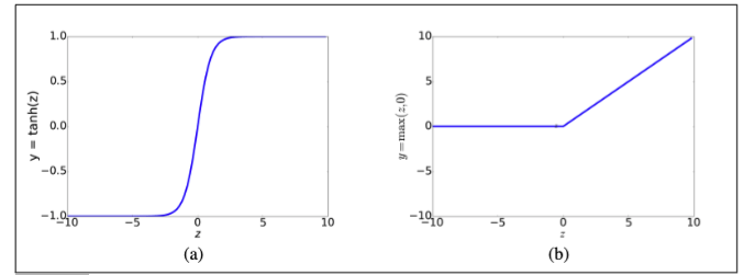
Tanh activation functions
ReLU activation functions
Neural Networks
Multi-layer Neural Networks (1/3)
Moving beyond single neurons by stacking multiple layers to form a Multi-Layer Neural Network.
Fully Connected (Dense) Architecture: The output of every neuron in one layer connects to every neuron in the following layer.
Mathematically, a neural network is a nested function.
$$y = \text{Softmax}(\text{Sigmoid}(\text{ReLU}(x \cdot w_1) \cdot w_2) \cdot w_3 + b_3)$$
Each layer applies a transformation followed by an activation function.
Neural Networks
Multi-layer Neural Networks (2/3)
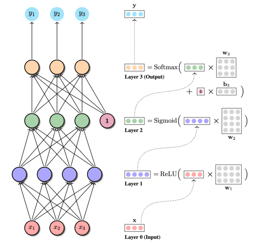
Output layer
Hidden layers
Input layers
Information Flow
Feed-forward Neural Networks (FFNNs)
Neural Networks
Multi-layer Neural Networks (3/3)
Model Depth: Measured by the number of layers with learnable parameters (hidden layers + output layer). The input layer is not counted, since it performs no computation.
-
Example: A network with an input layer, two hidden layers, and an output layer has a depth of 3.
Model Width: The number of neurons within a specific layer.
-
If all layers have \(n\) neurons, the model width is simply \(n\).
Universal Approximation: Even a 2-layer Sigmoid network can theoretically compute any function.
-
Deepening: For modern, "stronger" systems, increasing depth is generally favored over width for performance gains.
Introduction to NLP
Neural Networks Learn Through Feedback
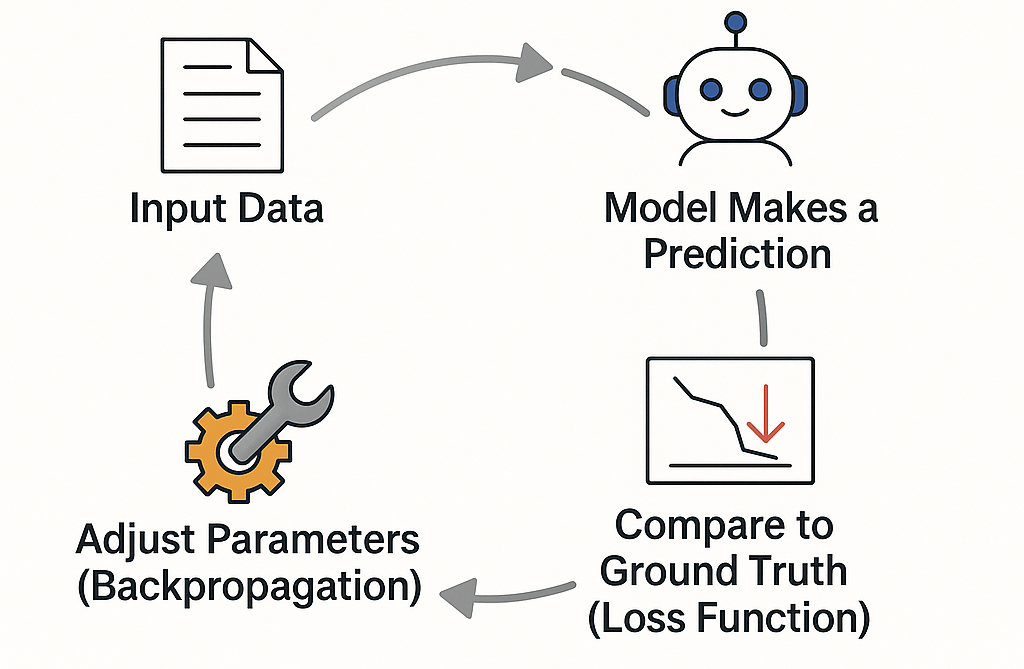
Neural networks learn through repetition: they make a guess, check how wrong it is, and adjust accordingly. Over time, guesses improve.
Neural Networks
Computation Graphs (1/3)
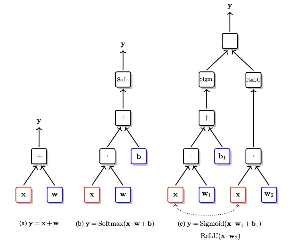
A computation graph is a directed graph that represents the mathematical operations of a neural network. It serves as a blueprint for the sequence of computations required to transform inputs into outputs.
Why use them?
-
They break down complex equations into simple, atomic steps.
-
They are the fundamental data structures used by deep learning frameworks (like PyTorch and TensorFlow) to manage computations.
-
They enable Automatic Differentiation (the ability to automatically calculate gradients).
Neural Networks
Computation Graphs (2/3)
Nodes (Vertices): Represent operations or variables.
-
Variables: Inputs (\(x\)), Weights (\(w\)), Biases (\(b\)).
-
Operations: Addition (\(+\)), Multiplication (\(\times\)), Activation functions (Sigmoid, ReLU).
Edges (Links): Represent the flow of data (tensors/scalars).
-
They carry the output of one node to the input of the next.
Direction: The graph is directed and usually acyclic (DAG), meaning data flows from input to output without loops (in feed-forward networks).
Neural Networks
Computation Graphs (3/3)
Neural Networks
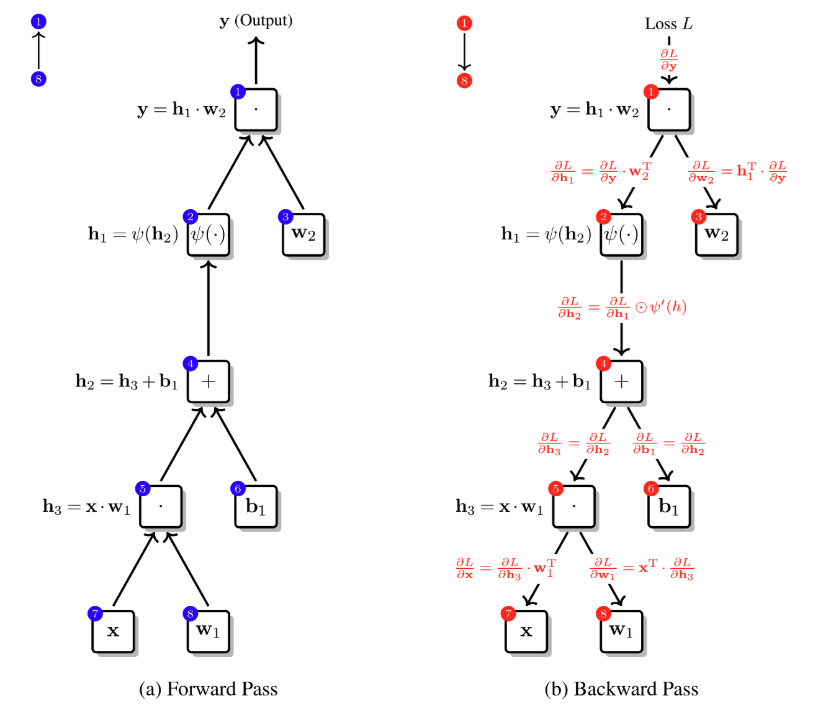
Forward Pass
Process: We traverse the graph from the input nodes to the output node.
At each node, we apply the specific operation to the incoming data.
Example: For \(y=\sigma(w\cdot x +b\)):
-
Compute \( u = w \cdot x\)
-
Compute \(z = u + b\)
-
Compute \( y = \sigma(z)\)
Result: The final node contains the prediction of the network.
Neural Networks
Backward Pass (1/3)
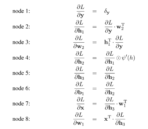
Goal: To train networks, we need partial derivatives of the Loss function \(L\) with respect to weights (\(w\)) and biases (\(b\)): \(\frac{\partial L}{\partial w}\) and \(\frac{\partial L}{\partial b}\).
Backpropagation:
-
Nodes are visited in reverse order (top-down).
-
Gradients are passed from the output back to the input.
Chain Rule:
-
For composite functions like \(y = p(q(x))\), we use the chain rule:
$$\frac{\partial y}{\partial x} = \frac{\partial p}{\partial q} \cdot \frac{\partial q}{\partial x}$$
Neural Networks
Backward Pass (2/3)
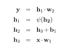
Let’s analyze the gradients for a specific function:
$$y = (x \cdot w_1 + b_1) \cdot w_2$$
We can decompose the function into several functions:
Neural Networks
Backward Pass (3/3)
Let’s analyze the gradients for a specific function:
Neural Networks
Example: Neural Language Modeling
Epochs and Steps
Training happens in cycles:
-
Epoch: one complete pass over the training data.
-
Step: One update to the model's weight.
Step 1
Step 2
Step 3
Batch
Batch
Batch
Batch
Epoch
A batch can consist of 8, 16, or 32 data examples.
Neural Networks
Why Do We Split the Dataset?
When working on a deep learning project, we split the dataset into:
-
Training set: used to train the model, update weights using loss and backpropagation.
-
Validation set: used to evaluate the performance during training, helps you tune hyperparameters like learning rate, number of layers, etc.
-
(Optional) Test set: used only at the very end, to evaluate final generalization.
Neural Networks
Regularization Methods
Why Generalization Matters?
A neural network learns from training data, but the goal is to perform well on unseen data.
Generalization: the model’s ability to apply learned patterns to new inputs.
In deep learning, this depends heavily on:
- Model architecture (layers, neurons)
- Number of parameters
- Size and diversity of training data
Neural Networks
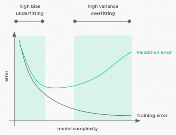
Underfitting: Model Too Simple to Learn
Happens when the network is not complex enough (e.g., too few layers or parameters).
Fails to capture patterns in data.
Results in:
- High training error
-
High test error
Causes:
- Shallow Network
- Not enough neurons
- Poor Feature representation
Neural Networks
Overfitting: Learn Noises, Not Just Patterns
Happens when the network is too complex relative to the data.
Models memorize training examples (and noises).
Results in:
- Low training error
-
High test error
Causes:
- Too many layers/parameters
- Small or noisy data
-
Long training without checks
Neural Networks
Bias-Variance Trade-off (1/2)
| Term | Description | Typically observed in |
|---|---|---|
| Bias | Error from overly simplistic assumptions; model fails to capture complexity | Neural network that is too shallow or has too few neurons (underfitting) |
| Variance | Error from excessive sensitivity to training data; model memorizes noise | Neural network that is overly deep/large relative to data (overfitting) |
-
In deep learning, model size directly affects this trade-off.
-
Goal: Minimize total error by finding the right model complexity.
Neural Networks
Bias-Variance Trade-off (2/2)
| Observation | Likely Cause |
|---|---|
| High train error, high test error | Underfitting |
| Low train error, high test error | Overfitting |
| Low train error, low test error | Good fit |
Always evaluate both training and validation loss.
Neural Networks
Why Do We Need Regularization?
Neural Networks
Neural networks can have millions to billions of parameters, which pose a risk of overfitting the data during training, causing them to memorize the data instead of generalizing.
Overfitting symptoms: Low training loss, high validation loss.
Goal of regularization: Promote simpler, more general models for better performance on unseen data.
L1 Regularization (Lasso)
Neural Networks
Adds a penalty proportional to the absolute value of weights to the loss function.
Goal: Reduce overfitting by shrinking less important weights to exactly zero (sparsity).
Feature Selection: Automatically removes irrelevant features.
Effect of \(\lambda\) :
- Small \(\lambda\) → less penalty, possible overfitting.
-
Large \(\lambda\) → more sparsity, high bias.
L2 Regularization (Weight Decay)
Neural Networks
Adds a penalty proportional to the square of the weights.
Goal: Shrinks all weights toward zero (but rarely exactly zero).
Distribute weight more evenly, especially with correlated features.
Effect of \(\lambda\):
-
Small \(\lambda\) → less penalty, possible overfitting.
-
Large \(\lambda\) → Stronger shrinkage, higher bias, lower variance.
Dropout (1/2)
Neural Networks
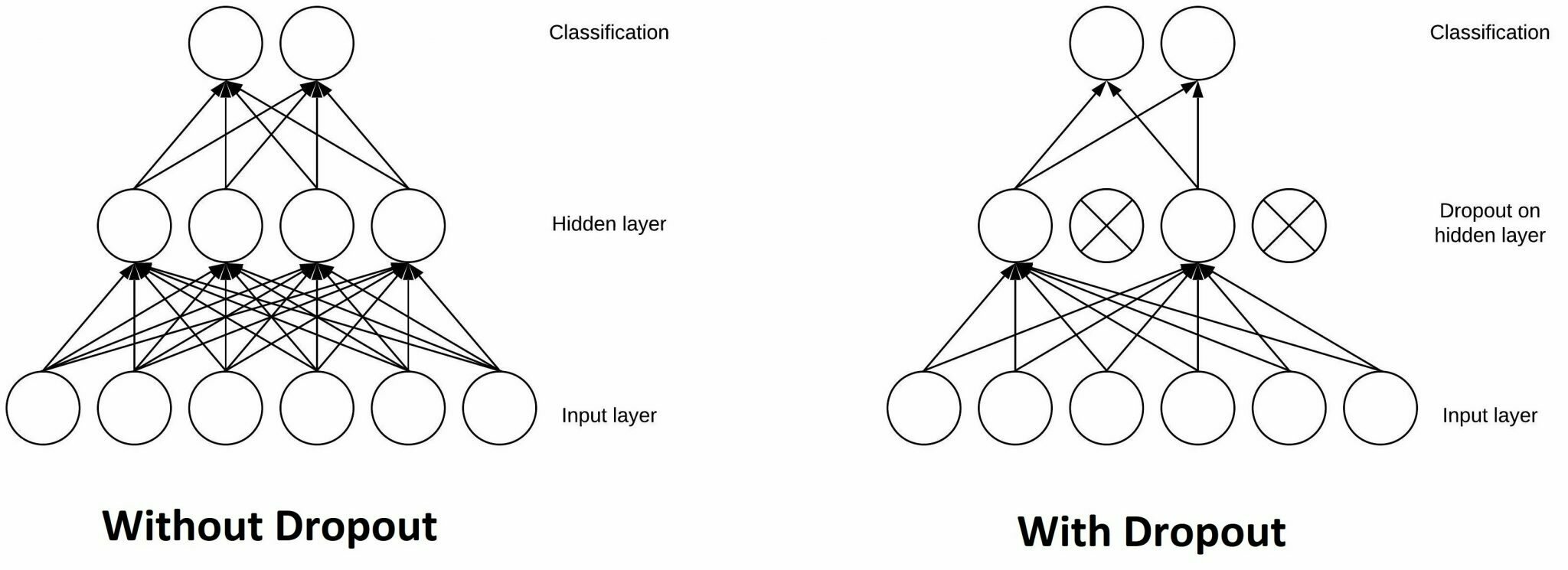
Randomly “drops” (sets to zero) a fraction of neurons during training to prevent overfitting
How it works:
-
At each training step, randomly deactivate a proportion p of neurons.
-
Dropout prevents the network from relying too much on specific neurons, encouraging more robust and distributed representations that improve generalization.
Typical Values: p = 0.2–0.5 (tuned via validation).
At Inference: No neurons are dropped.
Dropout (2/2)
Neural Networks
Early Stopping (1/2)
Neural Networks
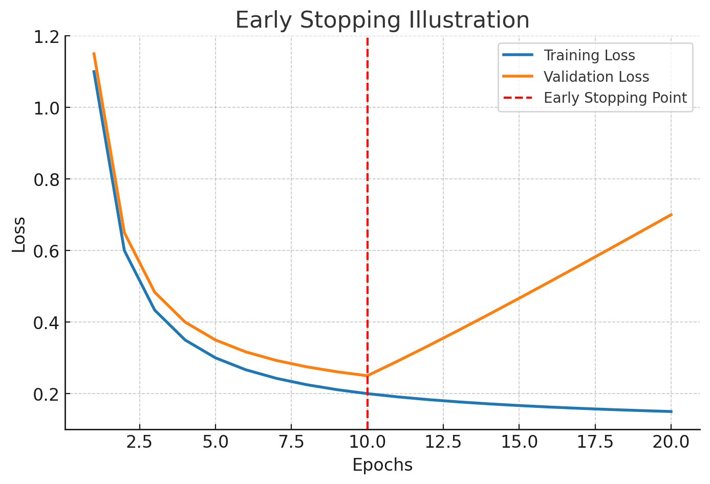
A regularization technique that halts training when performance on a validation set stops improving. This approach prevents overfitting by stopping before the model starts to memorize noise.
How it works:
-
Split data into training & validation sets.
-
Monitor validation loss/accuracy during training.
-
If validation performance does not improve for N epochs (patience), stop training.
Effect: Keeps the model near the point of best generalization.
Early Stopping (2/2)
Neural Networks
Data Augmentation (1/2)
Neural Networks
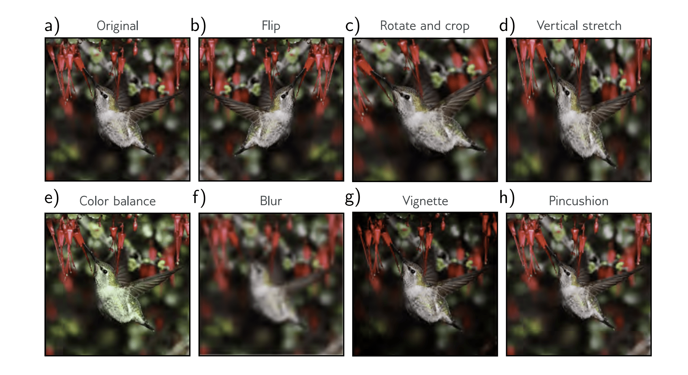
A regularization technique that expands the training dataset by creating modified versions of existing data. This increases dataset size, enhances generalization, and reduces overfitting.
How it works: Apply label-preserving transformations to data.
-
For images: rotations, flips, crops, color jitter, noise.
-
For text: synonym replacement, back translation.
-
For audio: pitch shift, time stretch, noise addition.
Effect: Improves robustness by exposing the model to varied but realistic inputs.
Data Augmentation (2/2)
Neural Networks
Optimization Algorithms
Gradient Descent with Momentum (1/2)
Neural Networks
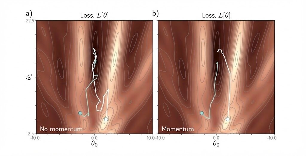
Treats parameter updates like moving an object through space, accounting for the "mass of motion" (momentum). It retains a portion of the previous momentum, preventing the velocity from becoming too large when approaching the minimum.
An advanced variant, Nesterov momentum, calculates the gradient after applying the previous momentum for better anticipation.
The Update Rule (Classic Momentum):
$$v_t = \lambda \cdot v_{t-1} - lr \cdot \frac{\partial L(\theta_t)}{\partial \theta_t}$$
$$\theta_{t+1} = \theta_t + v_t$$
The velocity vector of the momentum
A scalar weighting the previous momentum
Gradient Descent with Momentum (2/2)
Neural Networks
AdaGrad (Adaptive Gradient Descent)
Neural Networks
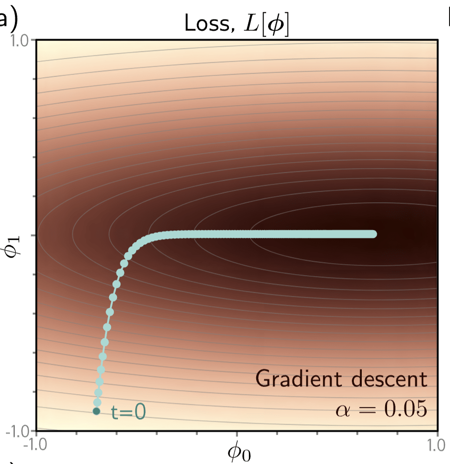
Instead of a global learning rate, AdaGrad adapts the learning rate for every single parameter.
It scales up the learning rate for parameters that are rarely updated and scales it down for parameters that are updated frequently.
The Update Rule:
$$G_t = \sum_{i=1}^t \left[ \frac{\partial L(\theta_i)}{\partial \theta_i} \right]^T \cdot \frac{\partial L(\theta_i)}{\partial \theta_i}$$
$$\theta_{t+1} = \theta_t - \frac{lr}{\sqrt{diag(G_t) + \epsilon}} \odot \frac{\partial L(\theta_t)}{\partial \theta_t}$$
Accumulation of the outer product of past gradients
A smoothing factor added for numerical stability.
AdaDelta
Neural Networks
AdaGrad's unweighted accumulation of past gradients can cause the learning rate to shrink too aggressively.
AdaDelta fixes this by replacing the unweighted sum with a moving average, using a decay factor to reduce the impact of "old" gradients.
The Update Rule:
$$g_t^2 = \sigma \cdot g_{t-1}^2 + (1-\sigma) \cdot \left( \frac{\partial L(\theta_t)}{\partial \theta_t} \odot \frac{\partial L(\theta_t)}{\partial \theta_t} \right)$$
$$\theta_{t+1} = \theta_t - \frac{lr}{\sqrt{g_t^2 + \epsilon}} \odot \frac{\partial L(\theta_t)}{\partial \theta_t}$$
decay factor strictly less than 1
Adam (1/2)
Neural Networks
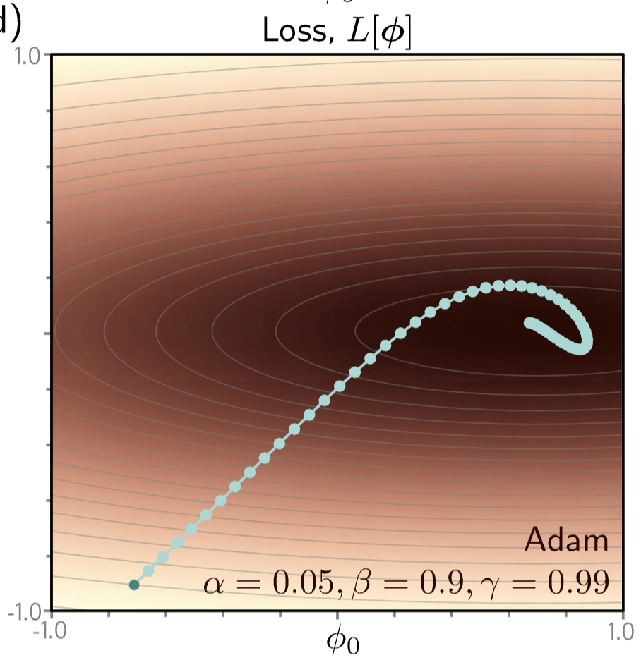
Adam (Adaptive Moment Estimation) is an optimizer that combines momentum (smoother, faster updates) with adaptive learning rates (per-parameter step sizes), providing stable and efficient training out of the box.
Adam remembers recent gradient directions (like momentum) and scales steps by recent gradient magnitudes (like RMSProp), which reduces noisy zig-zags, speeds convergence, and handles sparse or uneven features.
Adam (2/2)
Neural Networks
Other Optimization Algorithms
Neural Networks
There are many optimization algorithms designed to improve how neural networks learn.
All are based on gradient descent, but each adds its own twist.
Other optimization algorithms:
-
AdamW
-
RMSProp
-
Nadam
Hands-on Using Pytorch
What is Pytorch?

-
Open-source machine learning library.
-
Developed by Facebook’s AI Research Lab (FAIR).
-
Offers dynamic computation graphs (eager execution).
-
Widely used in both research and production.
Neural Networks
PyTorch Ecosytem




Neural Networks
Tensors
Neural Networks
Pytorch Installation
- Recommended: Use
condaorpip -
Install CPU-only:
- For GPU (CUDA):
- Visit https://pytorch.org/get-started/locally/
pip install torch torchvision torchaudioInstalling PyTorch is easy! First, ensure Python is installed, then use your terminal to install it.
Neural Networks
Let's Build a Neural Network
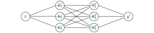
2 hidden layers of 3 neurons
Output layer
Input layer
Neural Networks
Step 1 - Prepare Data
import torch
from torch.utils.data import TensorDataset, DataLoader

x = torch.linspace(-1, 1, 100).unsqueeze(1)
y = 2 * x + 1

dataset = TensorDataset(x, y)-
Generates 100 points between -1 and 1.
-
Applies a known linear function.
-
Wraps inputs/targets as a dataset.
Neural Networks
Step 2 - Train/Test Split + Batching
from torch.utils.data import random_split, DataLoader

train_set, test_set = random_split(dataset, [80, 20])
train_loader = DataLoader(train_set, batch_size=10, shuffle=True)
test_loader = DataLoader(test_set, batch_size=10)
-
80/20 train-test split.
-
Enables batching using
DataLoader. -
Shuffles training data to improve learning.
Neural Networks
Step 3 - Define the Model
import torch.nn as nn

model = nn.Sequential(
    nn.Linear(1, 3),
    nn.ReLU(),
    nn.Linear(3, 3),
    nn.ReLU(),
    nn.Linear(3, 1)
)
-
Use
torch.nn.Sequential -
Input: 1D (x)
-
Hidden layers: 3 neurons with ReLU
-
Output: 1D (y)
Neural Networks
Step 4 - Define the Loss and the Optimizer
criterion = nn.MSELoss()
optimizer = torch.optim.SGD(model.parameters(), lr=0.01)-
Loss: Mean Squared Error for regression
-
Optimizer: Stochastic Gradient Descent
-
Learning rate: 0.01
Neural Networks
Step 5 - Train the Model
for epoch in range(100):

    for bx, by in train_loader:

        pred = model(bx)
        loss = criterion(pred, by)
        optimizer.zero_grad()
        loss.backward()
        optimizer.step()
-
Trains for 100 epochs.
-
Each epoch iterates over batches.
-
Backpropagation + gradient update.
Neural Networks
Step 6 - Evaluate on Test Data
model.eval()

with torch.no_grad():

    total_loss = 0

    for bx, by in test_loader:

        pred = model(bx)
        total_loss += criterion(pred, by).item()

print(f"Test MSE: {total_loss / len(test_loader):.4f}")-
No gradients computed during evaluation.
-
Aggregates test loss across batches.
Neural Networks